illuminAI

We must not fly too close to the sun or the sea.

You might know the Greek myth of Daedalus and Icarus: renowned craftsman Daedalus manufactures flying contraptions to allow him and his son Icarus to escape from their imprisonment by King Minos of Crete. Despite his father's stern warnings, Icarus flies so high that the heat of the sun melts the wax by which his wings were bound. He plummets towards the sea and drowns.

The (uncanonical) lesson I would like to extract is twofold: (1) the ability to interpret the internal mechanisms of a technology can save lives, and (2) such understanding involves the ability to reliably predict atypical behaviours of the technology.

Consider the following more concrete example: early deep learning models for detecting COVID-19 from chest radiographs were discreetly influenced by confounding factors.¹ The models struggled to generalize across different hospitals² and exhibited minimal changes in diagnoses after the lungs in X-ray image inputs were obscured,³ suggesting that their predictions weren't even based on the lungs at all! This genre of cautionary tale has become tragically real; in critical applications such as healthcare, strong test performance is marred by a lack of trust or understanding.

I. Towards interpretable AI

We define interpretability to be the degree to which a human can understand the cause of a decision.⁴ A COVID-19 diagnosis without any human-friendly justification is only partially helpful; a clear explanation of the decision makes it easier to validate the diagnosis and if necessary, to treat the patient. An equally robust definition which does not suffer from the difficulty of measuring understanding would be the degree to which a human can consistently predict the model’s result.⁵ If sixteen-year-old Icarus was fluent in Bayesian statistics and could predict his ornithopter's malfunction, he would surely not fly so close to the sun. More broadly, interpretable machine learning can offer insight into data beyond predictions, which can facilitate ethical AI design, alignment, and policy-making; ensure data privacy; increase training efficiency; decrease hallucinations; and help us steer clear of a future governed by accountability sinks in the form of blackbox models.

How can we increase the interpretability of our machine learning models? Is it simply hopeless once a model exceeds a certain threshold of computational complexity? Although many powerful models are not interpretable by design (e.g. neural networks), we can take inspiration from unit testing. In particular, it is generally wise to write tests which cover several typical inputs as well as any edge cases where the code unit risks producing a pathological output.

Inspired by this simple rule for software testing, we will illustrate a technique for cultivating interpretability called prototypes and criticisms. It will represent a model-agnostic, post hoc approach, which means it can be applied to any model irrespective of its architecture, at any point after the model is trained. Such generality sacrifices the possibility of exploiting the specific architecture of a model, but its flexibility across existing models and future innovations in machine learning is a virtue.

II. The prototypes and criticisms algorithm

As foreshadowed, prototypes constitute a subset of training points which are especially "representative" of the training set's overall distribution. By identifying prototypes, we obtain a summary of the dataset via concrete examples, which can yield key observations of our model's typical predictions. A classical algorithm for selecting prototypes is the $k$-medoids method. However, knowing prototypes can be of limited use if we wish to interpret the model's predictions for data points which are underrepresented in the set of prototypes. We call such outliers criticisms; examples are given in Figure 1 below.

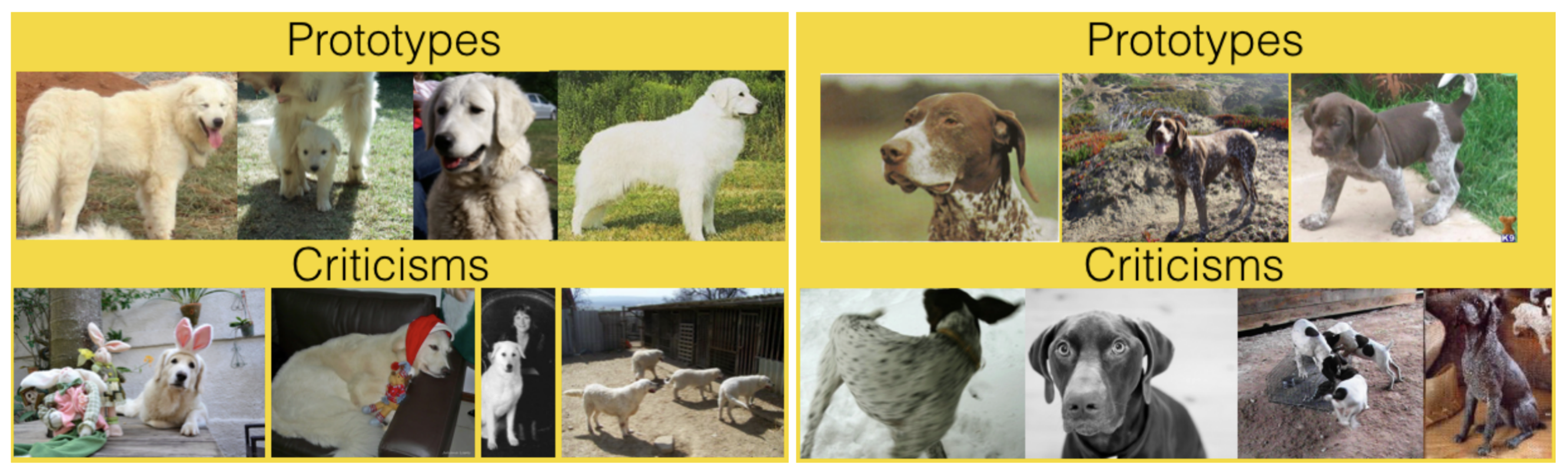
Figure 1: Learned prototypes and criticisms from the ImageNet dataset, for two dog breeds. Taken from ⁵.

The prototypes and criticisms heuristic can be formulated as follows:

1. Decide the number of prototypes and criticisms we want to find.

2. Select prototypes so that their distribution is "similar" to the data distribution.

3. Select criticisms at points where the distribution of prototypes maximally "differs" from the distribution of the data.

This vague procedure is bottlenecked by a precise notion of similarity or difference between the distributions of the prototypes and the entire dataset. We devote the next section to developing this concept.

II.1. The maximum mean discrepancy

We would like to measure the distance between two probability distributions, namely the prototypes and the entire dataset. Consider the following more general problem:

Problem: Let $x$ and $y$ be random variables on $\mathcal{X}$ with respective distributions $p$ and $q$. Given independently and identically distributed samples $X = {x_1,\dots,x_m}$ and $Y = {y_1,\dots,y_n}$ from $p$ and $q$, respectively, can we determine whether $p = q$?

Suppose $\mathcal{X}$ is a topological space, so it makes sense to discuss continuous functions on $\mathcal{X}$. If $\mathcal{X}$ is moreover a locally compact Hausdorff space (these are just niceness conditions for the topology on $\mathcal{X}$, and in practice not too difficult to come across), then it is a simple consequence of the difficult Riesz–Markov–Kakutani representation theorem⁶ that

$$p = q \quad \text{if and only if} \quad \mathbb{E}_x[f(x)] = \mathbb{E}_y[f(y)]$$

for all $f \in C(\mathcal{X})$, the space of bounded continuous real-valued functions on $\mathcal{X}$. In practice, the class of functions $C(\mathcal{X})$ can be arbitrarily large, rendering this criterion hopeless to compute. But as luck would have it, we can narrow our sights to any class $\mathcal{F}$ of functions $\mathcal{X} \to \mathbb{R}$ by defining the maximum mean discrepancy (MMD)⁷ of $p$ and $q$ with respect to $\mathcal{F}$ as

$$\tag{II.1.1}\mathrm{MMD}{\mathcal{F}}[p, q] = \sup{f \in \mathcal{F}} \left(\mathbb{E}_x[f(x)] - \mathbb{E}_y[f(y)]\right).$$

A priori, we may not know the distributions $p$ and $q$, so the following empirical MMD gives a sufficiently good estimate:

$$\tag{II.1.2}\mathrm{eMMD}{\mathcal{F}}[p, q] = \sup{f \in \mathcal{F}} \left( \frac1m \sum_{i=1}^m f(x_i) - \frac1n \sum_{j=1}^n f(y_j) \right).$$

MMD allows for a choice of class of functions $\mathcal{F}$, thus providing a more flexible measure of distance between the distributions $p$ and $q$. In the next section we construct and justify a common choice for $\mathcal{F}$.

II.2. Reproducing kernel Hilbert spaces

This section is fairly technical. Caveat lector.

Starting with a kernel function, we will construct a class of functions $\mathcal{F}$. It will turn out that the MMD with respect to this class $\mathcal{F}$ is particularly informative and readily computable in terms of the kernel.

A function $k \colon \mathcal{X} \times \mathcal{X} \to \mathbb{R}$ is called a symmetric positive-definite kernel on $\mathcal{X}$ if it satisfies the following properties:

1. For any $x_1,x_2 \in \mathcal{X}$, we have $k(x_1,x_2) = k(x_2,x_1)$.

2. For any $x_1,\dots,x_n \in \mathcal{X}$ and any $c_1,\dots,c_n \in \mathbb{R}$, we have

$$\sum_{i=1}^n\sum_{j=1}^n c_ic_jk(x_i,x_j) \geq 0.$$

In down-to-earth terms, a kernel can be thought of as a notion of similarity between points which can be realized as the inner product of some richer auxiliary space. More precisely, a result due to Moore and Aronszajn⁸ states that a symmetric positive-definite kernel on $\mathcal{X}$ determines a unique vector space $\mathcal{H}$ of functions $\mathcal{X} \to \mathbb{R}$ such that

• $\mathcal{H}$ is a Hilbert space, i.e. it is equipped with a "nice" inner product $\langle \cdot, \cdot \rangle \colon \mathcal{H} \times \mathcal{H} \to \mathbb{R}$.

• For each $x \in \mathcal{X}$, the function $k(x, \cdot) \colon \mathcal{X} \to \mathbb{R}$ is a vector in $\mathcal{H}$.

• For all $f \in \mathcal{H}$, $f(x) = \langle f, k(x, \cdot) \rangle$.

A particularly nice consequence of the last property is that

$$\tag{II.2.1}k(x,y) = \langle k(x, \cdot), k(y, \cdot) \rangle \quad \text{for all } x,y\in\mathcal{X}.$$

A vector space $\mathcal{H}$ arising in this way is called a reproducing kernel Hilbert space (RKHS). It turns out that the unit ball

$$\mathcal{F} = {f \in \mathcal{H}: \langle f, f \rangle \leq 1}.$$

in a RKHS $\mathcal{H}$ is generally a nice class of functions for computing MMD. Namely, the MMD with respect to $\mathcal{F}$ can fully determine distributions:

$$\mathrm{MMD}_{\mathcal{F}}[p,q] = 0 \quad \text{if and only if} \quad p = q.$$

Furthermore, the supremum in the definition of $\mathrm{MMD}_{\mathcal{F}}[p,q]$ will always be attained by some function $f^* \colon \mathcal{X} \to \mathbb{R}$, called the witness function. Following some calculations, we can express the witness function in terms of the kernel, up to a scalar:

$$\tag{II.2.2}f^*(z) \propto \mathbb{E}_x[k(x,z)] - \mathbb{E}_y[k(y,z)],$$

or for the empirical estimate,

$$\tag{II.2.3}\tilde{f}^*(z) \propto \frac1m\sum_{i=1}^m k(x_i,z) - \frac1n \sum_{i=1}^n k(y_i,z).$$

After normalization, we can and will assume that the exact equality holds in $(\mathrm{II}.2.2)$ and $(\mathrm{II}.2.3)$. As we can see in Figure 2, the witness function measures the signed difference between two distributions:

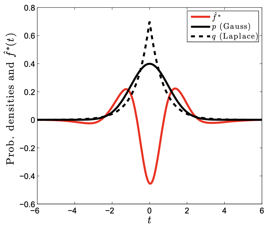
Figure 2: The witness function (red) measuring the discrepancy between a Gaussian distribution (solid) and a Laplace distribution (dashed). Taken from ⁷.

As we would like to measure their absolute difference, we substitute into $(\mathrm{II}.1.1)$ and $(\mathrm{II}.1.2)$ and then square to obtain

$$\tag{II.2.4}\mathrm{MMD}{\mathcal{F}}^2[p, q] = \mathbb{E}{x,x' \sim p}[k(x,x')] - 2\mathbb{E}{x \sim p, y \sim q}[k(x,y)] + \mathbb{E}{y,y' \sim q}[k(y,y')],$$

or empirically

$$\tag{II.2.5}\mathrm{eMMD}{\mathcal{F}}^2[p, q] = \frac1{m^2} \sum{i,j=1}^m k(x_i,x_j) - \frac{2}{mn} \sum_{i=1}^m \sum_{j=1}^n k(x_i,y_j) + \frac{1}{n^2} \sum_{i,j=1}^n k(y_i,y_j).$$

It remains to deploy this easily computable formula in our selection of prototypes and critics.

II.3. The MMD-critic algorithm

The following algorithm is due to Kim et al.⁵ To find the set of $k$ prototypes that best represents the distribution of the dataset, it suffices to find a subset $P \subset \mathcal{X}$ of cardinality $k$ that minimizes $\mathrm{MMD}{\mathcal{F}}^2[X, P]$. We can pick this subset with a simple greedy search, starting with an empty set of prototypes $P$ and adding the data point that minimizes $\mathrm{MMD}{\mathcal{F}}^2[X, P]$ when added to $P$. Our choice of $\mathcal{F}$ to be the unit ball in a RKHS makes it relatively easy to perform these computations using $(\mathrm{II}.2.4)$.⁹

To select criticisms, we interpret the witness function, which is approximated by

$$\tag{II.3.1}\tilde{f}^*(z) = \frac1m\sum_{i=1}^m k(x_i,z) - \frac1n \sum_{i=1}^n k(p_i,z),$$

where the $x_i$ are sampled from $X$ and the $p_i$ are sampled from $P$. In light of $(\mathrm{II.1.1})$ and $(\mathrm{II.2.1})$, this can be thought of as the difference between the average proximity of $z$ to the data and the average proximity of $z$ to the prototypes. If $\tilde{f}^(z)$ is near zero, then the distributions of the data points $x_i$ and the prototypes $p_i$ must be close together, hence $z$ would be a poor criticism. On the other hand if $\tilde{f}^(z)$ is very negative, then the prototype distribution overfits the data distribution. Finally, if $\tilde{f}^*(z)$ is very positive, then the prototype distribution underfits the data distribution.

This suggests that finding strong criticisms amounts to finding the points $z \in \mathcal{X}$ which maximize $|\tilde{f}^*(z)|$ . This can once again be implemented by a greedy search.

II.4. Limitations

The crucial limitation of prototypes and criticisms is the algorithm's sensitivity to various choices, some of them rather arbitrary. As we saw, prototypes and criticisms are mathematically quite distinct, but in practice their distinction is highly sensitive to the number of prototypes and criticisms we select. In general, there is no simple way to decide these numbers, and the optimal numbers vary across different applications. Similarly, the choice of kernel function is both a strength and a weakness, as each choice carries assumptions about the distribution of data, and determines the space of functions used to compute the MMD.

II.5. Implementations

• The original implementation of Kim et al. can be found on GitHub.

• A pip-installable Python implementation by Matthew Chak can be found at mmd-critic.

III. Applications to interpretability

Now that we understand the MMD-critic technique in detail, we consider its implications for interpretable machine learning.

Knowing prototypes and criticisms can improve our understanding of a dataset and its distribution, which certainly helps us decipher the model's decisions. Even better, we can examine the model's predictions for the prototypes and criticisms to obtain a concise summary of representative examples as well as outliers.

Additionally, given a prediction model $f$, we can use prototypes to construct a surrogate model $s$ that is interpretable by design and exhibits similar behaviours as the given model. A very simple surrogate model could take the form

$$s(x) = f(\mathrm{arg} , \max_{p \in P} k(x, p)),$$

replacing each prediction by the prediction corresponding to the nearest prototype.

The prototypes and criticisms methodology is remarkably simple. While the MMD-critic implementation relies on the deep theory of reproducing kernel Hilbert spaces, it represents a computationally feasible and extremely general method for cultivating interpretability in any machine learning model. As progress in artificial intelligence accelerates, it is essential that the rudiments of ethical AI design remain resilient in spite of paradigm shifts and the winds of economic pressure. Distinguished among these rudiments is the necessity of interpretability, where our capacity to understand the decisions of machine learning algorithms largely determines our ability to use these technologies for good.

References